- 07_비모수통계 (goodness-of-fit, gomogeneity, independence)
07_비모수통계 (goodness-of-fit, gomogeneity, independence)
Nonparametric statistics
모수통계 vs 비모수통계 특징
모수통계
모집단의 분포에 관해 특별한 가정을 세운 다음 통계적 추론을 시도하는 것을 말함
1) 추론의 대상이 모평균, 모비율, 모분산 등과 같은 모집단의 특성치, 즉 모수(parameter)라는 점
2) 추론방법이 비교적 엄격한 가정을 전제로 하고 있다는 점
비모수통계
1) 검정하고자 하는 가설이 모수와 관련된 것이 아닌 경우로서 적합도 검정이나 독립성 또는 동일성 검정, 표본의 무작위성 검정 등이 여기에 속함
2) 모집단의 분포가 명확하지 않아서 모수 통계방법을 사용하기 곤란할 때로서 모수통계의 대안으로 가정을 전제로 하지 않는 비모수 통계방법을 이용
3) 자료가 서열(rank)을 나타내는 순위자료이거나 순수한 범주적 자료일 경우
4) 간편한 방법으로 짧은 시간 내에 검정결과를 알고자 하는 경우
유형
적합도
1) RUN 검정: 표본 배열이 무작위로 구성되어 있는지 검정
2) Kolmogorov-Smirnov 검정(one sample): 표본의 분포가 가정한 분포를 따르는지 검정
동질성
1) Wilcoxon Signed-Rank Test(부호 순위 검정): 두 paired 표본의 부호와 서열로 분포를 비교 (paired t-test)
2) Mann-Whitney U 검정: 두 독립표본이 같은 분포를 따르는지 비교 (independent t-test)
3) Kruskal-Wallis H 검정: 2 집단 이상의 독립표본 집단의 분포 비교 (one-way Anova)
4) Friedman 검정: 3 집단 이상의 paired 표본 집단의 분포 비교 (two-way Anova)
상관성
1) spearman 서열상관 계수: 서열 또는 비율 척도 자료로 평가대상간의 일치성 검정
2) Kendall 서열상관 계수: 서열 또는 비율 척도 자료로 평가대상간의 일치성 검정
적합도 goodness-of-fit
RUN 검정
표본 배열이 무작위로 구성되어 있는지 검정
hypothesis: H0 (null) is that The data was produced in a random manner
syntax: runstest_1samp(x, cutoff=’mean’ or ‘median’, correction=True)
result: z-test statistic, p-value
from statsmodels.sandbox.stats.runs import runstest_1samp

#create dataset
data = [12, 16, 16, 15, 14, 18, 19, 21, 13, 13]

#Perform Runs test
runstest_1samp(data, correction=False)

# p값 0.50233이므로 0.05보다 크므로 귀무가설 수용, z-test statistic: -0.67082임
(-0.6708203932499369, 0.5023349543605021)
Kolmogorov-Smirnov 검정
표본의 분포가 가정한 분포를 따르는지 검정
hypothesis: H0 (null) is that The data come from a normal distribution
syntax: one sample은 scipy.stats.kstest(), two sample은 scipy.stats.ks_2samp()
result: statistic, pvalue
from numpy.random import seed
from numpy.random import poisson

seed(0)

#generate dataset of 100 values that follow a Poisson distribution with mean=5
data = poisson(5, 100)

from scipy.stats import kstest

#perform Kolmogorov-Smirnov test
kstest(data, 'norm')

# 포아송 분포로 추출했고 p값 1.0908062873170218e-103이므로 귀무가설 기각
KstestResult(statistic=0.9072498680518208, pvalue=1.0908062873170218e-103)
from numpy.random import randn
from numpy.random import lognormal

#generate two datasets
data1 = randn(100)
data2 = lognormal(3, 1, 100)

from scipy.stats import ks_2samp

#perform Kolmogorov-Smirnov test
ks_2samp(data1, data2)

# standard normal이랑 lognormal로 추출했고, pvalue 4.417521386399011e-57이므로 귀무가설 기각
KstestResult(statistic=0.98, pvalue=4.395433779467016e-55)
동질성 homogeneity
Wilcoxon Signed-Rank Test
두 paired 표본의 부호와 서열로 분포를 비교 (paired t-test)
두 paired 표본의 차이를 나타내는 분포가 정규분포를 따르지 않을 때, 모평균의 차이가 있는지
hypothesis: H0 (null) is that there is a no difference in the data between the two groups
혹은 the mean data is equal between the two group
syntax: wilcoxon(x, y, alternative=’two-sided’, ‘less’ or ‘greater’)
result: t statistic, pvalue
# mpg by new fuel treatment
group1 = [20, 23, 21, 25, 18, 17, 18, 24, 20, 24, 23, 19]
group2 = [24, 25, 21, 22, 23, 18, 17, 28, 24, 27, 21, 23]

import scipy.stats as stats

#perform the Wilcoxon-Signed Rank Test
stats.wilcoxon(group1, group2)

# 양측검정으로 p값이 0.044이므로 mpg가 같다는 귀무가설 기각
C:\Users\Administrator\anaconda3\lib\site-packages\scipy\stats\morestats.py:2967: UserWarning: Exact p-value calculation does not work if there are ties. Switching to normal approximation.
  warnings.warn("Exact p-value calculation does not work if there are "


WilcoxonResult(statistic=10.5, pvalue=0.044065400736826854)
Mann-Whitney U 검정
두 독립표본이 같은 분포를 따르는지 비교 (independent t-test)
sample 크기가 30보다 작고, 표본분포가 정규분포를 따르지 않을 때, 두 독립표본의 차이가 있는지
hypothesis: H0 (null) is that there is a no difference in the data between the two groups
syntax: mannwhitneyu(x, y, alternative=’two-sided’, ‘less’ or ‘greater’)
result: t statistic, pvalue
# mpg by new fuel treatment
group1 = [20, 23, 21, 25, 18, 17, 18, 24, 20, 24, 23, 19]
group2 = [24, 25, 21, 22, 23, 18, 17, 28, 24, 27, 21, 23]

import scipy.stats as stats

#perform the Mann-Whitney U test
stats.mannwhitneyu(group1, group2, alternative='two-sided')

# 양측검정으로 p값이 0.21138945901258455이므로 mpg가 같다는 귀무가설 기각
MannwhitneyuResult(statistic=50.0, pvalue=0.21138945901258455)
Kruskal-Wallis H 검정
2 집단 이상의 독립표본 집단의 분포 비교 (one-way Anova)
세 독립표본의 평균간에 차이가 있는지
hypothesis: H0 (null) is that the median is equal across all groups
syntax: stats.kruskal(a,b,c)
result: statistic, pvalue
# plant measurement
group1 = [7, 14, 14, 13, 12, 9, 6, 14, 12, 8]
group2 = [15, 17, 13, 15, 15, 13, 9, 12, 10, 8]
group3 = [6, 8, 8, 9, 5, 14, 13, 8, 10, 9]

from scipy import stats

#perform Kruskal-Wallis Test
stats.kruskal(group1, group2, group3)

# p값이 0.043114289703508814이므로 세 plant growth의 중앙값은 다르다
KruskalResult(statistic=6.287801578353988, pvalue=0.043114289703508814)
Friedman 검정
3 집단 이상의 paired 표본 집단의 분포 비교 (two-way Anova)
3 집단 이상의 평균이 통계적으로 유의미한 차이가 있는지
hypothesis: The mean for each population is equal
syntax: stats.friedmanchisquare(a), b, c)
result: statistic, pvalue
# response times for patient on each of the three drugs
group1 = [4, 6, 3, 4, 3, 2, 2, 7, 6, 5]
group2 = [5, 6, 8, 7, 7, 8, 4, 6, 4, 5]
group3 = [2, 4, 4, 3, 2, 2, 1, 4, 3, 2]

from scipy import stats

#perform Friedman Test
stats.friedmanchisquare(group1, group2, group3)

# p값이 0.0012612201221243594이므로 평균 반응시간이 다른다
FriedmanchisquareResult(statistic=13.351351351351344, pvalue=0.0012612201221243594)
상관성 (독립성) independence
서열 또는 비율 척도 자료로 평가대상간의 일치성 검정
ex) 값이 1,2,3,9999 여도 어차피 1,2,3,4 순위로 판단
Spearman Rank Correlation 서열상관 계수
hypothesis: H0 (null) is that correlation coefficient is 0.
syntax:
result: rho
-1: a perfect negative relationship between two variables
0: no relationship between two variables
1: a perfect positive relationship between two variables
, p-value
# math, science exam score of 10 students
import pandas as pd

#create DataFrame
df = pd.DataFrame({'student': ['A', 'B', 'C', 'D', 'E', 'F', 'G', 'H', 'I', 'J'],
                   'math': [70, 78, 90, 87, 84, 86, 91, 74, 83, 85],
                   'science': [90, 94, 79, 86, 84, 83, 88, 92, 76, 75]})

from scipy.stats import spearmanr

#calculate Spearman Rank correlation and corresponding p-value
rho, p = spearmanr(df['math'], df['science'])

#print Spearman rank correlation and p-value
print(rho)

# -0.41818181818181815이므로 음의 상관관계 존재

print(p)

# p값이 0.22911284098281892이므로 그렇게 significant 하진 않음
-0.41818181818181815
0.22911284098281892
kendall 서열상관 계수
kendall_서열상관계수 kendall_추가예제 spear만과 비교해서 표본이 적고, 동점이 많을 때에는 켄달 타우 계수 사용
x1 > x2 and y1 > y2 or x1 < x2 and y1 < y2 -> 일치 x1 > x2 and y1 < y2 or x1 < x2 and y1 > y2 -> 불일치
hypothesis: H0 (null) is that correlation coefficient is 0. syntax: kendalltau(x, y) result: corr, p-value
from scipy.stats import kendalltau

# 권위주의적성격(X)과 지위추구성향(Y)
X = [1, 2, 3, 4, 5, 6, 7, 8, 9, 10, 11, 12] # [x1, x2, x3, ...]
Y = [1, 3, 6, 2, 7, 4, 5, 10, 11, 8, 9, 12] # [y1, y2, y3, ...]


# Calculating Kendall Rank correlation
corr, _ = kendalltau(X, Y)
print('Kendall Rank correlation: %.5f' % corr)

# 0.0.69697이므로 X와 Y의 순위 상관은 비교적 높다고 판단
Kendall Rank correlation: 0.69697
연관성분석 Association analysis
특징
- 어떤 상품이 함께 팔리는가를 분석함으로써 경향성을 파악
- 연관규칙(if->then)을 통해 A 제품을 구매하는 사람이 n% 확률로 B제품을 구매하는지 확인
- 연관성 규칙의 종류
- 행동 가능한 규칙: 룰의 의미가 이해되고 실행이 바로 가능한 정보 ex) 물-라면, 기저귀-맥주
- 사소한 규칙: 이미 다 알고 있는 규칙으로 활용 관점은 낮지만 신뢰성 재확인 가능 ex) 삼겹살-상추
- 설명 불가능한 규칙: 설명되지 않고 실제 행동을 취할 수 없는 규칙 ex) 허리케인->딸기맛사탕
import warnings
warnings.warn('once')
import pandas as pd
import numpy as np
import matplotlib.pyplot as plt
import seaborn as sns
df_lotto = pd.read_csv('C:/Users/Administrator/Documents/Python/211120_ADP스터디/ADP/data/lotto.csv')
df_lotto.info()
<class 'pandas.core.frame.DataFrame'>
RangeIndex: 859 entries, 0 to 858
Data columns (total 7 columns):
 #   Column   Non-Null Count  Dtype
---  ------   --------------  -----
 0   time_id  859 non-null    int64
 1   num1     859 non-null    int64
 2   num2     859 non-null    int64
 3   num3     859 non-null    int64
 4   num4     859 non-null    int64
 5   num5     859 non-null    int64
 6   num6     859 non-null    int64
dtypes: int64(7)
memory usage: 47.1 KB
df_lotto.head()
| time_id | num1 | num2 | num3 | num4 | num5 | num6 | |
|---|---|---|---|---|---|---|---|
| 0 | 859 | 8 | 22 | 35 | 38 | 39 | 41 |
| 1 | 858 | 9 | 13 | 32 | 38 | 39 | 43 |
| 2 | 857 | 6 | 10 | 16 | 28 | 34 | 38 |
| 3 | 856 | 10 | 24 | 40 | 41 | 43 | 44 |
| 4 | 855 | 8 | 15 | 17 | 19 | 43 | 44 |
Transaction 데이터로 변환하기
1) melt를 사용하는 방법 (ADP 제공 패키지에 없음)
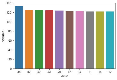
## transaction data로 변환 후 가장 많이 등장한 상위 10개 번호를 막대그래프로 뽑아내고 이에 대해 설명
melt = pd.melt(df_lotto, id_vars = ['time_id'])
melt.head()
| time_id | variable | value | |
|---|---|---|---|
| 0 | 859 | num1 | 8 |
| 1 | 858 | num1 | 9 |
| 2 | 857 | num1 | 6 |
| 3 | 856 | num1 | 10 |
| 4 | 855 | num1 | 8 |
pivot = melt.groupby('value')[['variable']].count().sort_values(by='variable', ascending = False)[:10].reset_index() #groupby시 variable에 count 값이 들어가고 index는 value인 pivot table
pivot.head()
| value | variable | |
|---|---|---|
| 0 | 34 | 134 |
| 1 | 40 | 126 |
| 2 | 27 | 126 |
| 3 | 43 | 125 |
| 4 | 20 | 124 |
sns.barplot(x = 'value', y = 'variable', data= pivot, order = pivot['value'])
plt.show()
2) mlxtend를 사용하는 법(ADP 제공 패키지에 존재)
http://rasbt.github.io/mlxtend/user_guide/preprocessing/TransactionEncoder/
from mlxtend.preprocessing import TransactionEncoder
## mlxtend는 list 속 list형식의 데이터를 One-hot encoding된 numpy array로 변환
list_lotto = df_lotto[df_lotto.columns[1:]].values.tolist() ## num1~num5 column의 value가 row마다 list형식으로 출력, 2d array를 tolist()로 리스트변환
te = TransactionEncoder()
te_ary = te.fit(list_lotto).transform(list_lotto) ##행:구매회차, 열: value(구매물품), 값: Boolean type 인 numpy 2d array
te_lotto = pd.DataFrame(te_ary, columns = te.columns_)

te_lotto.head()
| 1 | 2 | 3 | 4 | 5 | 6 | 7 | 8 | 9 | 10 | 11 | 12 | 13 | 14 | 15 | 16 | 17 | 18 | 19 | 20 | 21 | 22 | 23 | 24 | 25 | 26 | 27 | 28 | 29 | 30 | 31 | 32 | 33 | 34 | 35 | 36 | 37 | 38 | 39 | 40 | 41 | 42 | 43 | 44 | 45 | |
|---|---|---|---|---|---|---|---|---|---|---|---|---|---|---|---|---|---|---|---|---|---|---|---|---|---|---|---|---|---|---|---|---|---|---|---|---|---|---|---|---|---|---|---|---|---|
| 0 | False | False | False | False | False | False | False | True | False | False | False | False | False | False | False | False | False | False | False | False | False | True | False | False | False | False | False | False | False | False | False | False | False | False | True | False | False | True | True | False | True | False | False | False | False |
| 1 | False | False | False | False | False | False | False | False | True | False | False | False | True | False | False | False | False | False | False | False | False | False | False | False | False | False | False | False | False | False | False | True | False | False | False | False | False | True | True | False | False | False | True | False | False |
| 2 | False | False | False | False | False | True | False | False | False | True | False | False | False | False | False | True | False | False | False | False | False | False | False | False | False | False | False | True | False | False | False | False | False | True | False | False | False | True | False | False | False | False | False | False | False |
| 3 | False | False | False | False | False | False | False | False | False | True | False | False | False | False | False | False | False | False | False | False | False | False | False | True | False | False | False | False | False | False | False | False | False | False | False | False | False | False | False | True | True | False | True | True | False |
| 4 | False | False | False | False | False | False | False | True | False | False | False | False | False | False | True | False | True | False | True | False | False | False | False | False | False | False | False | False | False | False | False | False | False | False | False | False | False | False | False | False | False | False | True | True | False |
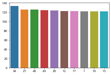
freq_lotto = te_lotto.sum(axis = 0).sort_values(ascending = False) ## axis=0이 column 기준으로 모든 row의 값을 더함, pd.Series로 return
sns.barplot(x = freq_lotto.index[:10].tolist(), y = freq_lotto.values[:10].tolist(), order = freq_lotto.index[:10].tolist())
plt.show()
연관규칙(Association Rule) 만들기
- Apriori algorithm이 사용되는 예시
- 신용카드 사기를 당했을 때 주로 결제되는 내역 패턴
- 암 발생 시 빈번히 나타나는 DNA 패턴과 단백질 서열 검사
- 빈도 평가 척도
- 지지도
- support(X) = n(X) / N
- support(X,Y) = n(X∩Y) / N
- 특정 아이템이 발생한 빈도
- 신뢰도
- confidence(X→Y) = n(X∩Y) / n(X)
- 아이템 X를 포함하는 거래 중 아이템 Y도 거래하는 비율
- 향상도
- lift(X→Y) = confidence(X→Y) / support(Y)
- Y 구매가 이루어진 확률 대비 X를 샀을 때 Y도 같이 살 확률
- lift가 1보다 클수록 +관계, 작을수록 -관계로 우연적 확률에서 멀어짐
- 지지도
## 기출문제) 최소지지도 0.002, 신뢰도 0.8, 최소조합 항목 수 2, 최대조합 항목 수 6 으로 설정한 연관규칙을 향상도 기준으로 내림차순 정렬하여 상위 30개 규칙을 확인
from mlxtend.frequent_patterns import association_rules, apriori
freq_items = apriori(te_lotto, min_support = 0.002, max_len = 6, use_colnames = True)  ## 이 두 개 조건밖에 지정이 안되는 듯?
freq_items  ## tuple 형태의 itemset - support(itemsets) 의 dataframe
| support | itemsets | |
|---|---|---|
| 0 | 0.142026 | (1) |
| 1 | 0.130384 | (2) |
| 2 | 0.129220 | (3) |
| 3 | 0.133877 | (4) |
| 4 | 0.138533 | (5) |
| ... | ... | ... |
| 6358 | 0.002328 | (40, 43, 13, 14, 26) |
| 6359 | 0.002328 | (14, 15, 18, 21, 26) |
| 6360 | 0.002328 | (40, 14, 27, 30, 31) |
| 6361 | 0.002328 | (34, 44, 15, 19, 21) |
| 6362 | 0.002328 | (36, 43, 16, 26, 31) |
6363 rows × 2 columns
freq_items['length'] = freq_items['itemsets'].apply(lambda x:len(x))  ## 조합항목 수 구하기

## 규칙 생성하기
rule1 = association_rules(freq_items, metric = "confidence", min_threshold = 0.8)  ## metric에 추가로 선택할 수 있는 leverage와 conviction은 뭔지 알아봐야 할 듯
rule1.sort_values(by = 'confidence', ascending=False)
| antecedents | consequents | antecedent support | consequent support | support | confidence | lift | leverage | conviction | |
|---|---|---|---|---|---|---|---|---|---|
| 0 | (1, 3, 43) | (12) | 0.002328 | 0.143190 | 0.002328 | 1.0 | 6.983740 | 0.001995 | inf |
| 1 | (1, 3, 15) | (25) | 0.002328 | 0.129220 | 0.002328 | 1.0 | 7.738739 | 0.002027 | inf |
| 464 | (26, 22, 14) | (44) | 0.002328 | 0.131548 | 0.002328 | 1.0 | 7.601770 | 0.002022 | inf |
| 465 | (35, 22, 14) | (39) | 0.003492 | 0.137369 | 0.003492 | 1.0 | 7.279661 | 0.003013 | inf |
| 466 | (14, 22, 39) | (35) | 0.003492 | 0.123399 | 0.003492 | 1.0 | 8.103774 | 0.003061 | inf |
| ... | ... | ... | ... | ... | ... | ... | ... | ... | ... |
| 236 | (32, 18, 6) | (31) | 0.002328 | 0.137369 | 0.002328 | 1.0 | 7.279661 | 0.002008 | inf |
| 237 | (34, 6, 31) | (18) | 0.002328 | 0.140861 | 0.002328 | 1.0 | 7.099174 | 0.002000 | inf |
| 238 | (18, 43, 31) | (6) | 0.002328 | 0.125728 | 0.002328 | 1.0 | 7.953704 | 0.002036 | inf |
| 239 | (43, 6, 31) | (18) | 0.002328 | 0.140861 | 0.002328 | 1.0 | 7.099174 | 0.002000 | inf |
| 703 | (16, 26, 31) | (43, 36) | 0.002328 | 0.012806 | 0.002328 | 1.0 | 78.090909 | 0.002298 | inf |
704 rows × 9 columns
## antecedents의 length를 새로운 데이터 column으로 빼서 그 값이 2와 6 사이인 데이터를 추출함
rule1['antecedents_len'] = rule1['antecedents'].apply(lambda x: len(x))
output = rule1[(rule1['antecedents_len']>=2) & (rule1['antecedents_len']<=6)]
output
| antecedents | consequents | antecedent support | consequent support | support | confidence | lift | leverage | conviction | antecedents_len | |
|---|---|---|---|---|---|---|---|---|---|---|
| 0 | (1, 3, 43) | (12) | 0.002328 | 0.143190 | 0.002328 | 1.0 | 6.983740 | 0.001995 | inf | 3 |
| 1 | (1, 3, 15) | (25) | 0.002328 | 0.129220 | 0.002328 | 1.0 | 7.738739 | 0.002027 | inf | 3 |
| 2 | (25, 3, 15) | (1) | 0.002328 | 0.142026 | 0.002328 | 1.0 | 7.040984 | 0.001998 | inf | 3 |
| 3 | (25, 3, 20) | (1) | 0.002328 | 0.142026 | 0.002328 | 1.0 | 7.040984 | 0.001998 | inf | 3 |
| 4 | (29, 3, 37) | (1) | 0.002328 | 0.142026 | 0.002328 | 1.0 | 7.040984 | 0.001998 | inf | 3 |
| ... | ... | ... | ... | ... | ... | ... | ... | ... | ... | ... |
| 699 | (16, 26, 43, 31) | (36) | 0.002328 | 0.133877 | 0.002328 | 1.0 | 7.469565 | 0.002017 | inf | 4 |
| 700 | (16, 43, 36) | (26, 31) | 0.002328 | 0.015134 | 0.002328 | 1.0 | 66.076923 | 0.002293 | inf | 3 |
| 701 | (16, 26, 36) | (43, 31) | 0.002328 | 0.018626 | 0.002328 | 1.0 | 53.687500 | 0.002285 | inf | 3 |
| 702 | (16, 26, 43) | (36, 31) | 0.002328 | 0.013970 | 0.002328 | 1.0 | 71.583333 | 0.002296 | inf | 3 |
| 703 | (16, 26, 31) | (43, 36) | 0.002328 | 0.012806 | 0.002328 | 1.0 | 78.090909 | 0.002298 | inf | 3 |
704 rows × 10 columns
## 향상도 기준으로 내림차순 정리
output.sort_values(by = 'lift', ascending = False, inplace = True)
output.head(30)
| antecedents | consequents | antecedent support | consequent support | support | confidence | lift | leverage | conviction | antecedents_len | |
|---|---|---|---|---|---|---|---|---|---|---|
| 703 | (16, 26, 31) | (43, 36) | 0.002328 | 0.012806 | 0.002328 | 1.0 | 78.090909 | 0.002298 | inf | 3 |
| 643 | (24, 34, 22) | (31, 7) | 0.002328 | 0.012806 | 0.002328 | 1.0 | 78.090909 | 0.002298 | inf | 3 |
| 642 | (34, 31, 7) | (24, 22) | 0.002328 | 0.012806 | 0.002328 | 1.0 | 78.090909 | 0.002298 | inf | 3 |
| 682 | (26, 21, 14) | (18, 15) | 0.002328 | 0.013970 | 0.002328 | 1.0 | 71.583333 | 0.002296 | inf | 3 |
| 652 | (34, 10, 36) | (44, 22) | 0.002328 | 0.013970 | 0.002328 | 1.0 | 71.583333 | 0.002296 | inf | 3 |
| 646 | (24, 22, 31) | (34, 7) | 0.002328 | 0.013970 | 0.002328 | 1.0 | 71.583333 | 0.002296 | inf | 3 |
| 666 | (24, 20, 15) | (12, 30) | 0.002328 | 0.013970 | 0.002328 | 1.0 | 71.583333 | 0.002296 | inf | 3 |
| 702 | (16, 26, 43) | (36, 31) | 0.002328 | 0.013970 | 0.002328 | 1.0 | 71.583333 | 0.002296 | inf | 3 |
| 700 | (16, 43, 36) | (26, 31) | 0.002328 | 0.015134 | 0.002328 | 1.0 | 66.076923 | 0.002293 | inf | 3 |
| 653 | (34, 10, 22) | (36, 44) | 0.002328 | 0.016298 | 0.002328 | 1.0 | 61.357143 | 0.002290 | inf | 3 |
| 658 | (26, 11, 36) | (17, 21) | 0.002328 | 0.016298 | 0.002328 | 1.0 | 61.357143 | 0.002290 | inf | 3 |
| 645 | (24, 31, 7) | (34, 22) | 0.002328 | 0.017462 | 0.002328 | 1.0 | 57.266667 | 0.002288 | inf | 3 |
| 676 | (26, 43, 13) | (40, 14) | 0.002328 | 0.017462 | 0.002328 | 1.0 | 57.266667 | 0.002288 | inf | 3 |
| 675 | (40, 26, 13) | (43, 14) | 0.002328 | 0.017462 | 0.002328 | 1.0 | 57.266667 | 0.002288 | inf | 3 |
| 636 | (45, 6, 31) | (18, 38) | 0.002328 | 0.017462 | 0.002328 | 1.0 | 57.266667 | 0.002288 | inf | 3 |
| 635 | (18, 45, 6) | (38, 31) | 0.002328 | 0.017462 | 0.002328 | 1.0 | 57.266667 | 0.002288 | inf | 3 |
| 664 | (12, 20, 15) | (24, 30) | 0.002328 | 0.017462 | 0.002328 | 1.0 | 57.266667 | 0.002288 | inf | 3 |
| 644 | (31, 22, 7) | (24, 34) | 0.002328 | 0.017462 | 0.002328 | 1.0 | 57.266667 | 0.002288 | inf | 3 |
| 701 | (16, 26, 36) | (43, 31) | 0.002328 | 0.018626 | 0.002328 | 1.0 | 53.687500 | 0.002285 | inf | 3 |
| 688 | (40, 14, 30) | (27, 31) | 0.002328 | 0.018626 | 0.002328 | 1.0 | 53.687500 | 0.002285 | inf | 3 |
| 665 | (12, 30, 15) | (24, 20) | 0.002328 | 0.020955 | 0.002328 | 1.0 | 47.722222 | 0.002280 | inf | 3 |
| 674 | (40, 13, 14) | (26, 43) | 0.002328 | 0.022119 | 0.002328 | 1.0 | 45.210526 | 0.002277 | inf | 3 |
| 694 | (19, 44, 21) | (34, 15) | 0.002328 | 0.024447 | 0.002328 | 1.0 | 40.904762 | 0.002271 | inf | 3 |
| 673 | (40, 43, 13) | (26, 14) | 0.002328 | 0.025611 | 0.002328 | 1.0 | 39.045455 | 0.002269 | inf | 3 |
| 667 | (20, 30, 15) | (24, 12) | 0.002328 | 0.027939 | 0.002328 | 1.0 | 35.791667 | 0.002263 | inf | 3 |
| 324 | (17, 14, 33) | (9) | 0.002328 | 0.103609 | 0.002328 | 1.0 | 9.651685 | 0.002087 | inf | 3 |
| 330 | (18, 35, 23) | (9) | 0.002328 | 0.103609 | 0.002328 | 1.0 | 9.651685 | 0.002087 | inf | 3 |
| 335 | (32, 43, 38) | (9) | 0.002328 | 0.103609 | 0.002328 | 1.0 | 9.651685 | 0.002087 | inf | 3 |
| 254 | (28, 7, 23) | (9) | 0.002328 | 0.103609 | 0.002328 | 1.0 | 9.651685 | 0.002087 | inf | 3 |
| 639 | (24, 34, 31, 7) | (22) | 0.002328 | 0.107101 | 0.002328 | 1.0 | 9.336957 | 0.002079 | inf | 4 |